


Average and its role in real estate appraisal
Canadian Property Valuation Magazine
Search the Library Online

By George Canning, AACI, P. App., Canning Consultants Inc., London, ON
There is no doubt that the average of any series of numbers is important. In his article entitled The Strange Power of the Idea of Average, published in the Financial Times on August 2, 2019, Tim Harford states that “It is the most radical statistical operation ever devised… The mean has a strange power over the way we think, and not always a benign one.”
Nobody knows who invented the arithmetic mean. It was used extensively in measuring observation and eliminating errors in one’s data. By the 1800s, just using an average was found to be a trap, since not all other observations in a given data set are errors or unimportant. In other words, there is value in understanding the mean of a set of numbers, but also the relationship of the mean to the other data points. While there are other types of means such as geometric, weighted, and harmonic, we are going to utilize the mean or average with which most valuers are familiar.
The biggest question for valuers is why they cannot take the average of a set of sales data and say that is the ‘market’ value of the property being appraised. There is no question that many valuers have gone down that path only to find it is fraught with errors.
As an illustrative point, I valued my house using sales after January 1, 2017, on similar cul-de-sacs in my neighbourhood. Graph 1 is the scatterplot of the sales data based upon the square footage of the sale houses.
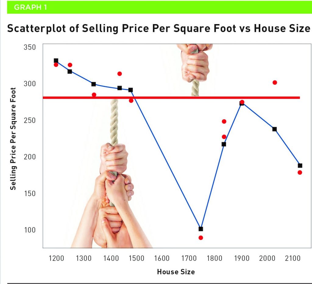
The red line is the average of the sales data at $258.09 per square foot of house. The blue line is a LOWESS Smoother. As the name implies, this is used to smooth out the shape of the data. But the Smoother is not so smooth, and it indicates a very erratic data shape. The average is being pulled by two groups of data. One is represented by the sales that occurred well below the average and the few sales above. They are outliers, and the characters are trying to pull this average to their advantage. We can say that our average is in trouble and that is because the data is quite skewed.
Some advocates would argue that the sales are older and they need to be time adjusted. We can turn to the published MLS statistics of the average prices of houses in London that sold in 2017, 2018, 2019 and 2020. With this information, we can determine an average annual increase in house prices that can be applied to the square footage of all the sales. Of course, using the average from an MLS database is completely wrong. The reason is that, in some years, there could be more houses selling that are priced lower than higher, which will affect the average for that year. The problem gets compounded from year to year because those years may have higher-end homes selling and vice versa. The skewing of the data set is still ever-present, even though we are dealing with a larger volume of sales. In the end, we are no further ahead in using unstandardized sales to value my house.
Others might say the problem is that the data is not normally distributed. What does that mean regarding sales data and the average?
The term normal distribution refers to a data set that is perfectly mirrored on either side of its average. It was invented by Carl Gauss in the 1800s and is also called the Bell Curve. Graph 2 indicates the normal distribution of data.
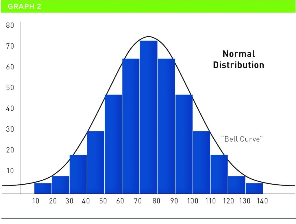
The normal distribution of data has amazing properties. The average, mode and median of the data in the distribution are equal. It can be used effectively for estimating and, historically, has been used by French card gamblers to increase their chances of winning. The curve does not touch the bottom of the graph because it is infinite.
If the sales data were normally distributed, the skewing is eliminated and, therefore, I should be able to use the average value of my house. The problem is that the data that forms the normal distribution is not the same as the subject property. The sales data needs to be adjusted for differences as a result of time, house size, lot size, condition, etc. The only way one can get around that problem is that the sales that form the normal distribution have to be an exact duplicate of the subject property. There is not much chance of that occurring.
At first glance, the use of the average of the selling prices of comparables is fraught with too many issues. The conclusion that could be reached is that it has no place in the appraisal process. However, that is not true. For example, if we want to use the average in the adjusted unit of comparison of comparable sales, we need to understand the role of two other statistical terms: standard deviation and coefficient of variance. Also, we need to condition our use of these two tools based upon an adjusted set of sales.
Knowing the average of anything is not very informative because one does not know the distribution or spread of the numbers that produced the average. If we said that the average house price in London, Ontario is $525,000, where the lowest selling house is $10,000 and the highest is $6,500,000, then the average has no meaning. Likewise, if the average was $525,000, where the lowest selling price was $475,000 and the highest was $575,000, then the average tells us more about the distribution pattern of the data. It becomes more meaningful.
Standard deviation is credited to Gauss. There is a quote on page 460 in the Anders Hald book A History of Mathematical Statistics from 1750 to 1930 that says: “The term Der mittlere Fehler (so named by Gauss) became standard in Germany, whereas in Britain no common terminology evolved before K. Pearson (1894) proposed the term ‘standard deviation’ adding in parenthesis as an explanation ‘error of the mean square.’ An error was replaced by deviation when the application of statistical methods spread to the social and biological sciences.”
One of the issues with statistical terms such as standard deviation is that it tends to get confusing. In very simple terms, standard deviation is the “distance around the mean that captures the majority of the sales in the data set.” Standard deviation is easily calculated by using an Excel spreadsheet. Here is an example. The average selling price of the comparables that I was going to use to value my house was $258.10. The standard deviation around that figure is $72.85. This means that the majority of the sales fell between $258.10 – $72.85 = $185.25 and $258.10 + $72.85 = $330.95. That is quite a spread. Using standard deviation on the raw data is a good indicator that the valuer has a long way to go to explain and reduce the variation in the data set.
The other term that is used with average is coefficient of variance (COV). Coefficient means number and variance is simply the difference or spread. We can calculate the COV by taking the standard deviation x 100% and divide it by the mean. In our case, the coefficient of variance percentage (COV%) is 28.22%. The COV% is crystallizing the average and the standard deviation into one singular number. This number is most critical and can be used as a fulcrum for valuation in the DCA.
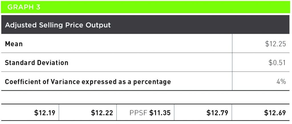
In quality point analysis, the whole DCA is focused on the COV. Here is an example taken from a recent appraisal of a converted office. Graph 3 indicates the adjusted selling price per square foot of building per point.
Within the QP spreadsheet, the mean, standard deviation, and COV are automatically calculated. It shows that the COV% is down to 4%. Given the fact that the unstandardized selling price range of the sales ‘going’ into the analysis was 55%, our valuation model with a COV% of 4% is starting to look good.
Graph 4 further demonstrates how the market value of the subject property was calculated using the average and the standard deviation.
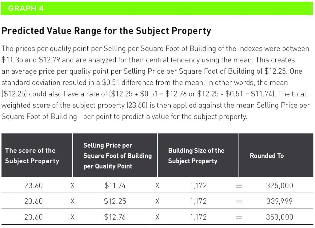
The standard deviation is the number that creates the range around the mean after adjustments. This makes sense because there needs to be some range in the potential value of the property since potential purchasers are not going to offer the same price.
It should be noted that standard-deviation around the mean has nothing to do with probability. It simply captures the distance around the average where the majority of the selling prices of the comparable fall (after adjustments). The lower the COV around that average is better because it means the adjusted selling price range is tighter.
The COV as a test to the reliability of using the average adjusted selling price of the comparables is a critical number. For example:
The adjusted selling price per square foot of commercial buildings is $100.00 – $120.00 – $135.00 – $150.00.
The average is $126.25 and the standard deviation is $18.49. By using COV%, it is 14.64%. We would suggest that the valuer go back to the drawing board to see if he or she can reduce the variance in the adjusted selling prices further.
However, what if the adjusted selling price per square foot of commercial buildings was $120.00 – $125.00 – $124.00 – $122.00 – $126.00? The average is $123.40 with a COV% of 2.15%.
Now this valuer has a more reliable model of valuation and can use the average of $123.40 as a means of value plus and minus the 2.15%. The value of the property would fall somewhere in this range.
We should not limit the use of average to the DCA. It is also applicable to overall capitalization rates and GIM. However, the latter has to be adjusted to make equal between the attributes of the subject property and that of the sales.
Conclusion
Using the unadjusted selling prices of comparable sales, no matter how perfect they seem, is a poor way to value real estate. There are always differences that need to be accounted for between the sales and the subject property. Also, most of the variance between the sales is not always visible on the surface and that is why a computer is needed for the adjustment process.
We can use the average as a reliable number on the following three conditions:
- The average unit of measure is after adjustments.
- The COV% has to be a low number, say under 5%.
- The property value range is going to be +- the COV% around the mean or average.
Some comments received from other valuers is that the COV% cannot be lower than 10%. Is there some standard number around the mean that should be an indicator of well-adjusted sales? The answer is no. If one cannot get a COV% of less than 5%, it might mean the wrong comparables are being used, the adjustments are incorrect, or, perhaps given the rarity of the property under valuation, a COV% around the mean of 10% is fine.