


Financial Leverage: A Double Edged Sword
Canadian Property Valuation Magazine
Search the Library Online
By JT Dhoot, AACI, P. App., CBV
Founder & Principal, Omnis Valuations & Advisory Ltd.
Members of the Appraisal Institute of Canada (AIC) are frequently asked to value real property for mortgage financing purposes. While real estate is appraised as though free and clear of mortgage financing, the current or anticipated amount of debt secured by a property impacts the financial risk accepted by a property owner and, by extension, the risk borne by the appraiser should the property owner default on the loan.
Valuation theory states that, all else equal, the rate of return demanded by an equity investor will increase as financial leverage increases. This means financial risk, defined as “risk related to the use of debt to finance an investment,” increases as an investor uses more and more debt.[1] Accordingly, a prudent investor will demand a higher expected rate of return as compensation for accepting incremental financial risk.
Valuation theory also states that, excluding the tax benefit arising from tax-deductible interest on debt, value cannot be created (or destroyed) by simply changing an asset’s capital structure. Stated differently, “The change in financial structure does not affect the amount or risk of the cash flows on the total package of the debt and the equity” and therefore “the market value of any [property] is independent of its capital structure.”[2] Be that as it may, appraisers must remember that “the transaction price for one property may differ from that of an identical property due to different financing arrangements[]” and thus “appraisers must make sure that cash equivalency adjustments reflect market perceptions” when this is the case.[3]
How much, if any, debt a property owner chooses to use in a particular situation depends on numerous factors, including but not limited to:
- the type, location, age, condition and use of the property;
- the property’s historical and, more importantly, anticipated cash flows;
- the property owner’s investment strategy, risk tolerance and financial resources; and
- the availability, terms and cost of debt including the covenants that, if breached, will cause the loan to be in default.
In contrast to financial risk, the terms market risk, operating risk and/or business risk are used broadly to describe shifts in supply and demand, changes in laws and regulations, fluctuations in capital markets, etc. Simply put, these factors impact the amount, timing and perceived risk(s) of the expected benefits (i.e., cash flows) anticipated from a property, irrespective of how the property is financed. In other words, the unlevered (also known as unleveraged, before-debt, debt-free or all-cash) cash flows anticipated from a property are not influenced by financial risk. The market risk, operating risk and/or business risk are factors that affect the selection of an appropriate terminal capitalization rate and discount rate but they are independent of financial risk, which is related solely to the impacts of financial leverage (i.e., debt).
In theory, “any shift in capital structure can be duplicated or “undone” by investors”[4] and for this reason, any financial risk a property owner chooses to accept will only impact the expected risk and return on her/his equity, not the expected risk and return on the asset as a whole (i.e., the total package of the debt and equity). Again, the caveat here is the property is not being transacted on the basis of atypical or non-market financing.
The following case study attempts to illustrate these concepts using a hypothetical commercial property and some simplifying assumptions:
- A 2,500 sq.ft. commercial property is purchased today for $1,000,000, based on a going-in overall capitalization rate of 5.0%.
- The property owner intends to hold the property for five years, with the estimated terminal value at the end of the holding period calculated using a terminal capitalization rate of 5.0% and assuming no transaction costs.
- In Year 2 and each year thereafter, the property’s Net Operating Income (NOI) is anticipated to change based on five distinct market scenarios (collectively, the ‘Market Scenarios’):
- Market Scenario 1 = NOI changes at a Compound Annual Growth Rate (CAGR) of -6%
- Market Scenario 2 = NOI changes at a CAGR of -3%
- Market Scenario 3 = NOI remains the same (CAGR = 0%)
- Market Scenario 4 = NOI changes at a CAGR of +3%
- Market Scenario 5 = NOI changes at a CAGR of +6%
- Each of the Market Scenarios is analyzed on the basis of three separate financing scenarios (collectively, the ‘Financing Scenarios’):
- Financing Scenario 1 = No financial leverage (Loan-to-Value or LTV ratio of 0%)
- Financing Scenario 2 = Moderate financial leverage (LTV ratio of 50%)
- Financing Scenario 3 = Significant financial leverage (LTV ratio of 85%)
- Each of the Market Scenarios assumes a vacancy and collection loss allowance and structural allowance of 0%.
- Each of the Financing Scenarios (except for Financing Scenario 1, which has no financial leverage) assumes the cost of debt is 3.0%, debt service is calculated using a 25-year amortization period, and the income tax rate is 0%.
Figure 1 illustrates the property’s forecasted NOI under each of the Market Scenarios. As a reminder, NOI is calculated on a before-debt and before-tax basis, which means that the Financing Scenarios do not influence the calculation of NOI.
Figure 1
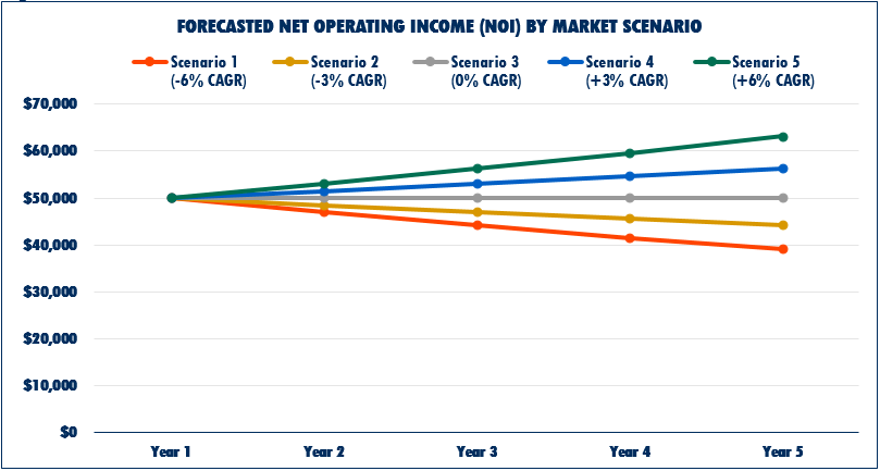
Figure 2 illustrates the property’s forecasted terminal value under each of the Market Scenarios. Again, the terminal capitalization rate and NOI are ‘unlevered’ metrics, which are not impacted by financial leverage (or income tax) and, therefore, the Financing Scenarios do not influence the terminal value calculations. Note that the property is forecasted to sell at a loss in Scenario 1 and 2 (due to declining NOI, coupled with no change to the capitalization rate), break-even in Scenario 3 (although it is technically incorrect to say ‘break even’ if the time value of money is considered), and at a gain in Scenario 4 and 5 (due to increasing NOI coupled with no change to the capitalization rate).
Figure 2
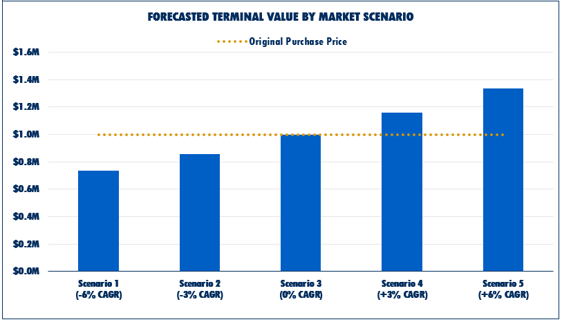
Figure 3 illustrates the forecasted Internal Rate of Return (IRR) on equity for each of the Market Scenarios and Financing Scenarios, or 15 scenarios in total (5 Market Scenarios x 3 Financing Scenarios = 15 total scenarios). This analysis illustrates the following:
- The IRR on an unlevered basis (i.e., no financial risk) ranges from a low of -1% to a high of 11% depending on the particular Market Scenario.
- The addition of financial leverage in Financing Scenario 2 results in the IRR range widening to a low of -5.5% and a high of 17.1%.
- Increasing financial leverage to 85% LTV under Financing Scenario 3 results in an indeterminate IRR on the low end (more on this later) and 35.0% on the high end.
Overall, both downside risk and upside potential are magnified as the use of financial leverage is increased.
Figure 3
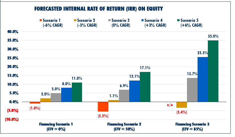
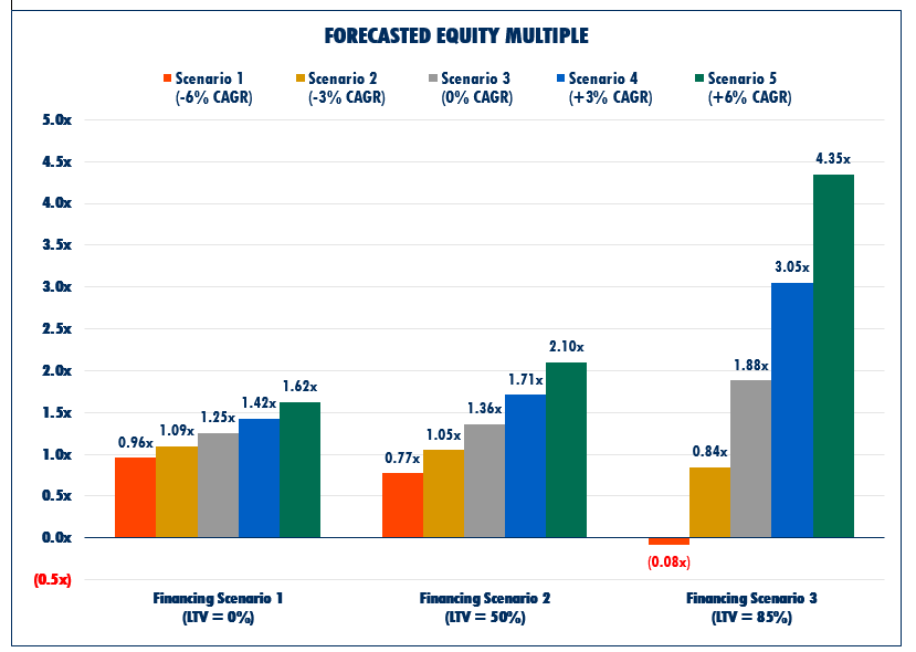
Figure 4 illustrates the forecasted equity multiple for each of the Market Scenarios and Financing Scenarios. The equity multiple is calculated by dividing the total equity cash flows received from an investment by the investor’s initial equity contribution. Although the equity multiple does not account for the time value of money, the risk profile of the income stream or the duration of the investment horizon, it does provide a relatively simple metric that answers the question “How many dollars will I get back for each dollar I invest?” An equity multiple greater than 1.0x indicates the investor will receive more than he/she invested, while an equity multiple lower than 1.0x indicates the investor will receive less than her/his initial investment. A negative equity multiple indicates the investor will lose more than the amount he/she originally invested.
As noted earlier, the combination of Market Scenario 1 and Financing Scenario 3 results in an indeterminate IRR. This is because the poor operating performance of the property (i.e., declining rental rates and NOI) coupled with high financial leverage (i.e., LTV=85%) creates a scenario where the equity investor suffers a loss in excess of her/his equity initial investment. In other words, the definition of IRR cannot be satisfied in this scenario, as there is no “discount rate that makes the net present value of all cash flows from a particular investment equal to zero.” Figure 4 indicates the equity multiple for Market Scenario 1 combined with Financing 3 results in an equity multiple of negative 0.8x, meaning the investor would suffer a total loss of her/his $150,000 initial equity investment and an additional loss of roughly $12,200 (calculated as $150,000 initial equity investment x equity multiple of negative 0.08x).
Figure 4
In summary, appraisers are well positioned to assist their clients in evaluating the risks and rewards of using financial leverage in real estate transactions. Members of the AIC who prepare appraisal reports for mortgage financing purposes can reduce their exposure to risk in these types of engagements by following best practices that include naming the authorized lender and potentially limiting the type and amount of financing for which the appraiser is willing to accept liability (i.e., first mortgage financing up to 75% LTV).
End notes
[1] The Appraisal of Real Estate, 3rd Edition, Editor: Larry Dybvig, Appraisal Institute of Canada, c2010, p. 5.6
2 Brealey, Richard A., Stewart C. Myers, and Franklin Allen. Principles of Corporate Finance. New York, NY: McGraw=Hill/Irwin, 2006.
3 The Appraisal of Real Estate, 3rd Edition, Editor: Larry Dybvig, Appraisal Institute of Canada, c2010, p. 14.11
4 Brealey, Richard A., Stewart C. Myers, and Franklin Allen. Principles of Corporate Finance. New York, NY: McGraw=Hill/Irwin, 2006.