


Loss of Use analysis: A fresh look at the Proxy Model
Canadian Property Valuation Magazine
Search the Library Online
By John E Farmer, P. App., AACI, MRICS, Q.Arb.; Gina Gallant, BComm, P. App., AACI; and Norris Wilson, BA, P. App., AACI
The famed astronomer Galileo Galilei said that mathematics is the language of the universe. He perhaps meant that mathematics is fundamental to our understanding of life. Professional Appraisers (P. App.) are well-versed in applying simple mathematical concepts which form the basis of appraisal.
In a simple example, if an appraiser found that a 10,000-square foot warehouse sold for $1 million, this transaction is distilled by basic division into a market indicator as such: $1,000,000 ÷ 10,000 square feet = $100 per square foot. Or, in other words, price divided by area equals unit rate per dollar. If that same property was generating $100,000 in annual net rent, the appraiser would then demonstrate, using simple division, that the ratio between the annual income and the sale price was a 10% return. Supposing that the income was perpetual, the investor would expect a 10% capitalization rate.
Historically, appraisers have been trained to consider equity return with an eye to the loan-to-value ratio and the return net of financing. Today, through the use of tools such as discounted cash flow (DCF) analysis software, calculations are more comprehensive. The power of DCF analysis is that it can employ numerous assumptions over a forecast timeline and convert future annual performance into a present value estimate in seconds.
In addition, today’s Professional Appraiser (P. App.) must work to comprehend the issues at play in a given valuation assignment. Using the universal language of mathematics, they can provide answers to complex questions.
Poignant examples can be found in cases where the complex issue of Loss of Use arises, such as in a First Nation land claim. Where questions arise such as ‘surrender of parts of original reserves,’ or ‘shortfall in treaty land entitlement,’ how can an appraiser use pure mathematical principles to calculate values?
Appraisers are familiar with the ‘principle of anticipation’ in real estate valuation: the idea that the property’s market value is the present value of the sum of anticipated future benefits. Returning to our earlier example of a property acquired for $1 million, with an anticipated income of $100,000 per year, and supposing that the income was derived from land rent instead of a warehouse building, the answer is still the same. The return is embodied in the 10% capitalization rate.
The Proxy Model is a variation of the land rental approach to value. In this case, the land rental rate is a proxy for the economic return for land which, when applied to the market value of the land, results in an estimate of nominal annual rent. The power of this technique is that the appraiser can point to any point in time and project the anticipated return for a given property or plot to the present day. Therefore, this estimated historical income stream is processed into a present value which, in theory, reflects compensation for the Loss of Use of the land over time.
What is Loss of Use?
The concept of value presumes that the purchaser/owner is motivated by future returns on their investment (i.e., enjoyment of living in their home, collecting rent from a tenant, raising livestock, harvesting a crop to sell at market, etc.). But what happens when that was taken away a century ago or more; how do you calculate what was lost?
The loss to an owner of a single tenant industrial property would be the lost rent for each year. Similarly, the landowner that has lost the use of their land is deprived of their ability to rent the land to a tenant. In each instance, not only has the owner been deprived of income, but, theoretically, that rental income could have been saved in a bank or invested, to generate financial returns.
The Proxy Model, therefore, is not only a means by which to consider the loss of revenue for each year, but also to calculate the loss of the return on that revenue for each year. Once these amounts have been calculated for the duration of the loss, this provides an insight into a claim for Loss of Use.
It may be argued that the landowner that suffered the loss could have used their revenue for their own purposes over time. But this stance simply ignores the reality that the owner was deprived of their ability to enjoy this revenue and never had the opportunity to deploy this revenue. Even if it had been spent rather than invested, economists agree that the future benefits arising from whatever the revenue was spent on would be at least as advantageous as saving the money in an investment account.
In applying the theory of the Proxy Model, the Loss of Use of the land is measured on the basis of imputed land rent foregone by the landowner over the period between the loss and present day. The foundation of the rates applied is based upon observations of market activity over this period and these represent the proxy for the losses endured.
Example scenario
A landowner in Alberta lost the use of their 1,000 acres of farmland on January 1, 1913. The price of land at that time was hypothetically $3,000 ($3.00 per acre). As of the date of loss, the land had been cleared and used for pasture and some crop production. It had been surveyed under the township system and patents registered at land titles.
At the present effective date, (December 31, 2020), the same 1,000 acres has a hypothetical current value appraised at $1,000 per acre. For the sake of simplicity, we will say that the land has not changed in terms of either use or development.
The following evaluates the compensation owed to the landowner from the date of loss to the current effective date.
General approach
There are four main components to the Proxy Model:
- Define land value at the date of Loss of Use 1(a) and the current date 1(b)
- Define annual growth rates in land value over time since 1(a)
- Define the return on the land (annual rental rate) for each year for the duration of the loss
- Define return on annual land rent proceeds received for each year as if it had been invested
The Proxy Model requires the estimation of several variables.
1(a) Retrospective value of the land
Establishing the value of land at a past date presents challenges to the appraiser; the further back in time the appraiser needs to delve, the greater the effort to complete diligent research into historical transactions.
For example, say the appraiser in Alberta has access to online records back to the mid-1980s. For earlier periods, requests must be made directly to the historical department of the land titles office. An added complication is that the province did not officially exist until April 1905, so historical transactions prior to 1905 need to be traced through federal archives, museum records, and other library sources.
The quality of the land is also something to establish as of the retrospective effective date. Early settlers to the western provinces were faced with land in a raw and natural state. This was advantageous if the homestead was in an area of grassland, but more challenging if it was covered in trees and the settlers needed to clear stumps or drain swampy low-lying areas. Either way, the price of the land from the government or railway company (liquidating their land holdings) would reflect the raw state.
An adjustment for clearing costs is then required to reflect the time and cost to bring the land into a productive state for agricultural purposes, a painfully slow and laborious process initially done without the help of modern machinery.
1 (b) Current value of the land
Establishing the current value of the land follows current valuation approaches, which are outside the scope of this article.
2 Estimating the annual change in land value between dates 1(a) and 1(b)
Once the values have been established at their respective points in time, it follows that there is an annual change in value over time between the two dates – historical and present.
The rate of annual change can be derived from empirical evidence. Several approaches have been used in past applications of the Proxy Model, including prorating the growth between the start and end value estimates on a straight-line basis, or using Canadian inflation, which may or may not give a result to match the current value estimate in the appraisal. Other time series have been estimated using inflation as measured by the Consumer Price Index for the period up to 1949 and then a rate which inflates the 1950 value forecast in a straight line to match the current appraised value, or by estimating retrospective value at points along the timeline, say every 25 or 30 years, and straight lining the projected value between these.
Generally, it is not believed that general inflation is a suitable guide to the fluctuations of land value over time. Estimating values at intermediate check-in dates is not always considered to be a practical solution either, as the choice of dates may miss important inflection points in the economy and result in over or under estimating the changes in value over time.
The authors recommend that the appraiser create a time series on which to base an imputed land rent cash flow. For example, Altus Group uses the long-term value trend indicated by the blend of provincial (post-1921, when Statistics Canada information became available) and Kansas farm value data (pre-1921). Using statistical rates provides a strong proxy for a logical growth rate.
The farm value time series is a general statistical trend used to provide the annual change in land values over time. Just using this series alone leaves the calculation vulnerable to a basic weakness — that the appraiser would be unable to link the retrospective date (1a) to the current date (1b). Therefore, the appraiser needs to buffer the value trend data with a constant, so that the annual inflator applied to 1(a) arrives at a unit value mathematically consistent with 1(b). The buffer constant is a fixed number that is calculated in the spreadsheet to align the time series to arrive at the current value (1b). This is a simple process with today’s spreadsheet technology.
Figure 1 provides an example (not all years shown):
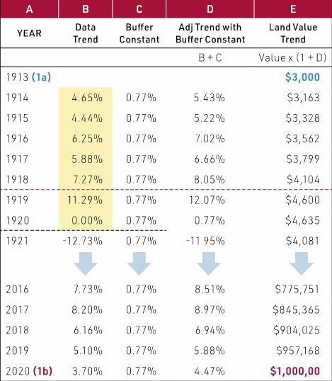
Figure 1 © Altus Group
Column A the effective years, between 1913 and 2020
Column B statistical farm value time series (Kansas to 1920, Stats Canada 1921 onwards)
Column C the buffer constant
Column D the adjusted statistical farm value time series
Column E the annual projected value of the land for each year of the timeline, arriving at the current value (1b)
Understanding how land prices have changed through time involves some basic understanding of history. For example, Statistics Canada has records going back to 1921. Since then, as shown in Figure 2, the agricultural economy was affected by a spike in farm value immediately after WW1, the downturn in the 1930s, increases in land value in the late 1960s when chemical fertilizer enhanced crop yields and profitability, and the downturn in the 1980s because of high inflation and interest rates, followed by generally increasing land prices up to present date.
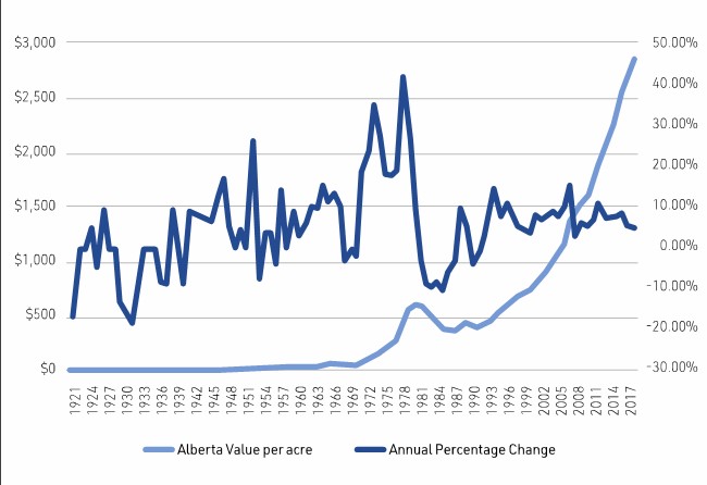
Figure 2 © Altus Group
To extend this back to the retrospective date, reference is made to the statistics on Kansas farm values which are available back to 1860. When the Alberta vs Kansas data is compared (between the available Alberta data 1921 and 2019), it is found that there is a strong correlation coefficient of 97%, as illustrated in Figure 3.
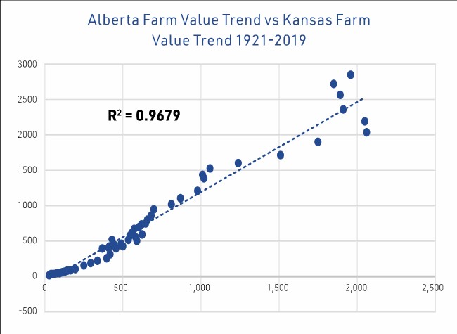
Figure 3 © Altus Group
This gives great confidence in using annual changes in Kansas farm values to backfill the period in the farm value trend series prior to 1921, back to the retrospective date (1a).
3 Annual land rental rate
This is the more challenging concept to understand, as there are two moving parts to the equation. First, the underlying assumption is that the Loss of Use of the land has led to a loss of revenue to the former owner. This needs to be calculated for each year of the duration of the loss. Second, it is assumed that this revenue would have been saved and invested in a savings account, accumulating compound interest.
At this point, it is important to remember that the point of the Loss of Use analysis is that the owner lost the use and revenue from their land every year. Because they never received that income, they never had the opportunity to make the revenue work for them, in whatever way they would have chosen to do so. Thus, the compensation claim using the Proxy Model assumes that this revenue would have been saved and would have earned interest in the intervening years.
Land rent estimate
Return on land is generally perceived as the residual yield after all the agents employed in the business on the land have been satisfied. In other words, the gross revenue from the business enterprise is allocated first to labour, then to capital, management and profit, and, finally, to land.
Land capitalization rates are the ratio between cash rent for land and the value of that land at a point in time. An example of the dynamic of this statistic is illustrated in Figure 4 based on statistics on land rents and land values for the State of Kansas produced by the USDA for the period from 1985 to 2009.
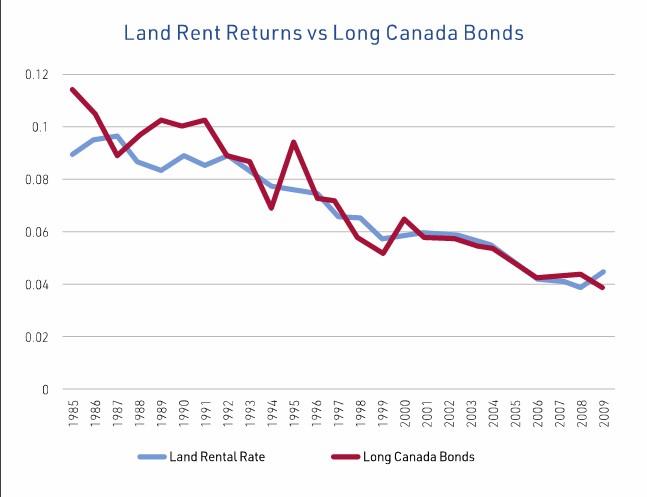
Figure 4
Source: Bank of Canada and USDA statistics
Due to the lack of a long-term series of such land rental rate data, the Kansas data was compared to several financial instruments to try to find a reasonable proxy for land rent returns that could be applied over a long period of history. Long Canada bonds are graphed against the available Kansas land rent series and there is a reasonable similarity between them over time.
To test this, we created a scatter plot (Figure 5) to investigate the degree of similarity between the two series and found a correlation coefficient of 0.86, which we regard as being reasonably similar. Taking into account the fact that long bond rates are among the lowest rates of return offered and are thus considered a ‘safe rate,’ the resulting rent estimates should be viewed as conservative.
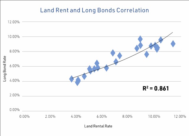
Figure 5 © Altus Group
Given the similarity between land rates of return and long Canada/US bond rates, long bond rates are used as a proxy for land capitalization rates used to estimate annual land rent amounts.
Part I: Bond rates
Past application of the model has used an inflation adjusted yield rate based on real return Canada bonds. The real return or ‘real rate’ concept is useful to gauge the effective return to the investor net of inflation, but no one would invest in a bond which did not provide some protection from future inflation.
In fact, the use of the face rate of return (real rate) only reflects part of the story of these investments.
The Canadian real return bond series, which some analysts have referred to for Loss of Use cases, does not simply return a rate of interest shown on the face of the bond but also adjusts the value of the bond at maturity for inflation in step with the Consumer Price Index. In truth, the actual return on a real return bond is a combination of the face interest rate and an adjustment for inflation to preserve the capital value of the investment. The correct rate of return to land must be one that includes inflation or at least a risk buffer for anticipated future inflation.
There is a problem, however, in that historical records of Canada long-term bond rates (10 years and up) are only available back to 1919. In order to supplement this time series for earlier periods previous to 1919, reference can made to a bond return series developed by US economics professor Robert Shiller. His data provides long bond interest rates back to 1871 for the US — but are they reasonably similar to Canada bonds?
Plotting the Canada series and the US series over their common history shows a strong correlation (Figure 6). The correlation coefficient derived from a scatter plot (Figure 7) on these series was over 0.96, which is considered statistically significant and indicates the two series moved in near perfect tandem over the study period. We conclude one can reasonably be substituted for the other.
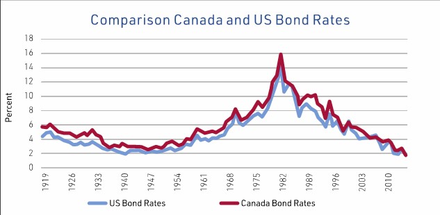
Figure 6
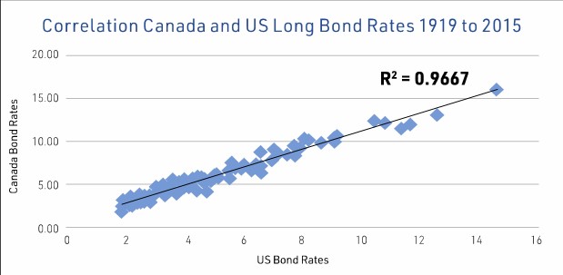
Figure 7
Source: Robert Shiller: US Long Bond Rates www.econ.yale.edu/~shiller/data.htm
Source: Bank of Canada Long Canada Bond Rates www.bankofcanada.ca/rates/interest-rates/canadian-bonds/
Therefore, if required, the appraiser can supplement the Canadian data from Statistics Canada with the US data for 1871 to 1918. Doing so provides the result shown (Figure 8).
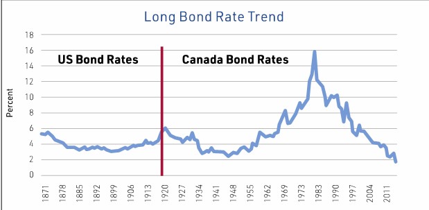
Figure 8
Source: Robert Shiller and Bank of Canada
To continue with this hypothetical example, rates of return are thus a blend of rates from the US (1913 to 1918) and then long Canada bond rates (Figure 9).
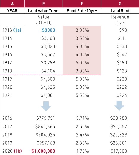
Figure 9 © Altus Group
Column E represents the annual land value (inflated over time to current value).
Column F represents the Bond Rate proxy for a rate of return from the land, with US data prior to 1918 and Canadian data from 1919 onwards.
Column G estimated annual land rent
Part II: Return on rent
In the normal course of business, it is expected that any land rent earned by a First Nation would have been deposited in a band trust account maintained by the Government of Canada and would earn the interest rates set over time by Indigenous Services Canada (ISC) and its precursors. In applying this model to a private sector situation, the assumption would be that a safe rate of return as represented by Canada long term bonds would be appropriate. The band trust account rate was prescribed by ISC up to 1969 and thereafter reflects Canada long bond rates, so relatively similar results can be expected.
Part III: Interest calculation
A December 2016 decision by the Specific Claims Tribunal (SCT) Huu-Ay-Aht First Nations v. Her Majesty the Queen in Right of Canada, 2016 SCTC 141 awarded Loss of Use compensation for timber revenue. The interest rate applied to the loss forecast was based on a blend of short- and long-term Canada bonds and the band trust rate. All the forecast foregone revenue was brought forward to current date on the basis of 100% compound interest.
Also, in December 2016, in Beardy’s & Okemasis Band #96 and #97 v. Her Majesty the Queen in Right of Canada, 2016 SCTC 15,2 the SCT awarded compensation for withheld annuity payments from 1885-1888 based on compound interest using the band trust fund rate.
Most recently, the decision in Southwind v. Canada, 2021 SCC 283 affirmed the use of compound interest in bringing loss of use nominal annual rent estimates forward to current date.
In keeping with these decisions, in our example we base our model on 100% compound interest at the band trust rate.
In Figure 10, the land rent (Column G) is invested at the band trust rate (Column H) to generate the annual interest on the rent saved.
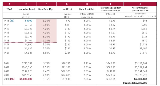
Figure 10 © Altus Group
Therefore, in 1913, the claimant would have received $90 in land rent (G) and banked $2.70 (I) interest at 3.0% band trust rate on $90, thus ±$93 (J).
In the following year (1914), the claimant would also receive land rent ($111) (G) and band trust rate interest of $3.32 (I). However, the accumulator column also reflects that the claimant would have had $93 in the bank that would gain interest at the band trust rate. Thus $111 + $93 ($203) is inflated by the band trust rate, resulting in $209.
Then in 1915, the land rent (G) is $133, which is added to the amount accumulated from the previous two years. This is inflated by the band trust rate. Thus ($133 + $209 = $343) x 1.03 = ±$353, and so on.
Once all years have been considered, the accumulated loss of value in the above hypothetical example would be $5,880,000, reflecting not only the loss of rent income, but also the loss of return on that rent.
Clearing costs and development
As noted earlier, the land may be in a raw state as of the retrospective date. The appraiser will need to research the cost and rate of clearing and reflect these in the model as well. It has been quoted by historians that a homesteader may be able to manage to clear 20 acres per year. Land granted to homesteaders was often on the basis that they could enter the land and, subject to their periodic clearing of the land, the balance of the purchase price would be due once the land was in an altered and productive state.
In some situations, the land in question may have been further subdivided and developed at later points in time. The appraiser needs to evaluate the cost of capitalizing on these periodic changes in highest and best use and make additions or deductions in the revenue forecast as a result and where appropriate.
Conclusion
The example featured in this article was simplified to illustrate the basic assumptions and calculations required for Loss of Use cases, but, in practice, the model can also be configured to account for costs of development for agriculture and for evolving land uses, as well as to reflect any income earned by a First Nation from sales proceeds from surrendered land over time.
It is equally important to coordinate the assumptions in the Loss of Use model and the changes in highest and best use of land over time with the valuation at current date to ensure that no double accounting takes place.
As you can see, the Proxy Model is theoretically sound and results in well supported estimates of Loss of Use compensation. However, this is only possible when credible estimates of land value, land rent, and investment returns are based on historical evidence which is relevant to the real estate market over long periods of time.
End notes