

The Application of Multivariate Regression Analysis in Expropriation Matters
Canadian Property Valuation Magazine
Search the Library Online


By George Canning, AACI, Canning Consultants Inc., London, ON
Injurious affection can be the most difficult form of land compensation to prove before any court of law. The claim for compensation is a right under the law, but that does not mean entitlement. In many cases, compensation is not quantifiable because of the insufficient quantities of data, the complexities of data analysis and the unfamiliarity with advanced methods needed to allow the data to ‘speak.’ In these cases, the right to compensation may conclude as ‘difficult to prove’ or ‘not enough data’ and, subsequently, be filed in the ‘still wondering’ cosmos of fragmented exploratory data analysis.
This article delves into the principle use of multivariate regression analysis as it relates to land compensation issues and a brief introduction about another form of data analysis when data tends to be ‘thin.’ It is intended to aid real estate practitioners wanting to use more advanced methods of data analysis in solving injurious affection claims. This is not a statement that the use of these tools will guarantee the claimant’s right to compensation, but they will give the real estate expert a more detailed look at the data when the paired sales method provides no useful conclusions.
Land compensation claims for such injurious affection issues as loss of parking, reduction in front yard setbacks, increased traffic flow, loss of view, subsurface rights and even application of the traditional ‘before’ and ‘after’ method are real estate problems that can be handled by using multiple regression analysis.
The problems of data analysis
Data is found in the marketplace and it tends to have irregular patterns of behaviour. What you think the data is trying to say and what is really occurring are often two separate issues. Without proper real estate data analysis, the answer to an injurious affection claim maybe buried beneath a pile of raw property attributes. In order to ‘clear the clutter,’ a multiple regression analysis ‘run’ may inform the real estate practitioner the true basis for the claim and the appropriate amount of settlement. Conversely, the claiming of ‘loss’ may not be present and becomes quite apparent through more ‘robust’ testing of the sales data.
The problem with real estate data stems from the fact it is unstructured and is both found in a numeric and a non-numeric format. However, the underlying function of real estate data analysis is to reduce uncertainty. The more certain that your real estate data is behaving in a particular way, the better the decisions regarding its value, or the particular effect a property variable is having on explaining injurious affection loss.
Regression analysis is not perfect, but it has strong attributes that make this a desirable option regarding substantiating injurious affection claims or their denial.
First, it helps one to organize the data and allows for the exploration of the most rudimentary form of data analysis: graphing. The following is a good example of using graphs to help describe data. However, caution is required since visual presentations can be misleading.
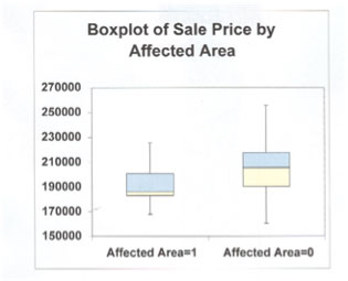
The red lines in the above box plot are the average selling price of two sets of data. One is land that is affected by a contaminant and the second is without. The observation is that land affected sold for approximately $187,000, while the non-affected land sold for $205,000. After applying all the property attributes to the date set, it was concluded that there was little difference in price. Here are some cautionary notes. Numeric data analysis should go hand in hand with a visual presentation of the data. An arguable point is the reverse of that statement. The use of an average price from a grouping of data only without the graph is dangerous. Seeing the shape of the data might suggest that average is not a meaningful number and the more appropriate expression would be the median or mode. That is why no appraiser should rely on ‘the average yearly price of houses sold’ from any MLS system, for example. The average number given is just a number.
This number becomes more relevant when the boundaries of the average price and the attributes that cause these differences to occur are known. It is like saying “all land is the same because it is just dirt.”
Second, it can be used to explore the relationship between variables. As appraisers, we sometimes think certain variables are the ones that drive various types of real estate property prices. By simply exploring your data through a regression program, you may find the opposite to be quite true. Income is not always the driving force behind ‘income producing properties,’ for example. Sometimes, data attributes can interact with one another and result in displays of property characteristics never possibly imaged. However, similar property attributes can throw the data picture off because one is trying to dominate the other.
Third, the most striking feature of multiple regression analysis is its ability to hold constant all variables while it explores each single variable independently.
Although the regression analysis formula can be expressed in several different ways, its basic function has not changed since it was invented by Sir Francis Galton in 1820.
Y= AX + B
Here, the above equation can be modified to add countless variables as follows.
Y=a+b1*X1 +b2*X2 +…
The b1*X1 could represent house size, while the b2*X2 could represent house age. It can go to infinity and the number of variables used in the equation is directly related to the amount of data. That is what makes regression analysis such a powerful data tool. As the model assigns a coefficient or number to each variable, it holds all others still. It would be the equivalent of freezing five house sales and the appraiser walking in each house and observing a plaque card for each property attribute with its value written upon it.
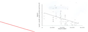
Below is a case dealing with the ‘taking’ of a road widening. In this expropriation matter, there were two injurious affection possibilities or potential claims: (1) a loss in value because of a decrease front yard setback, and (2) a loss in value as a result of increased traffic flow. The following graphs denote a distinct pattern to these claims.
Traffic
Setback
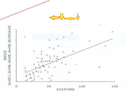
The graph on the left shows the regression line with a negative slope as traffic counts increase from left to right. While traffic counts are increasing, sale price on the ‘Y’ axis is decreasing. The graph on the right shows the regression line with a positive slope as setbacks decrease along the ‘X’ axis from left to right. The corresponding sale price on the ‘Y’ axis shows a decrease in value as setbacks decrease. However, how does the actual data output match what the graphs are eluding to?
Output of the regression run
Regression analysis is not about making a red line through two sets of data. The above two graphs illustrate the relationship between two variables (setbacks and traffic volume) against sale price. It would be in error to draw a line up from traffic counts and then over to sale price for an indication of loss. That is an inaccurate method of analysis, because the above graphs are only telling us that there is a strong relationship between these two variables and sale price. Perhaps it is nothing more than a spurious relationship between setbacks and traffic volume against sale price. However, there are a number of other property characteristics that need to be included in the regression analysis that should form part of the ‘regression run’ that might also explain these relationships.
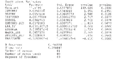
The following was the ‘regression run’ of the database, which consisted of 81 observations representing similar (not identical) properties to that of the subject property.
Traffic counts
The effect of traffic counts on the data is shown by the coefficient -6.729380E-6. The ‘T’ statistic is shown as -4.410. Both of these numbers are a negative because the increase in traffic volume is having a negative impact on sale price.
The ‘T’ statistic is simply a measure of significance. In other words, how confident is the valuer that the results of the coefficient -6.729380E-6 are statistically meaningful and did not appear simply by random chance? As a rule of thumb, a ‘T’ score greater than two would indicate that the outcome obtained is not due to random chance. This is verified by the p-value – 0.000. P values are probabilities and are generally set for a 5% level. A number above 5% would mean that the coefficient obtained by the regression model would have most likely appeared by chance. Therefore, a p-value below 5.0% would indicate that the coefficient was the result of something other than chance. The p-value of 0.000 for the traffic count coefficient is less than 5.0%
The -6.729380E-6 is in scientific notation and really means that, for every change in one traffic count, sale price decreased by .000006729380 dollars in sale price. If we use 10,000 cars as a base, this figure would change to 0.06729. If we wanted to convert this latter figure to a percentage, this number would be multiplied by 100% as follows: 0.06729 x 100% = 6.729% (round to 6.73%). This means that, for every change in 10,000 car traffic counts, sale price fell by 6.73%. In the case of the subject property, the traffic counts prior to the ‘taking’ are 23,000 cars per day, which will increase over time to 33,000 cars. This is a difference of 10,000 cars.
Therefore, the value of the subject property would be negatively impacted by 6.73%. There are two points to consider in the application of the 6.73% to the subject property. The first point is that the increase in traffic volumes will not occur immediately. This would mean that, at the effective date of the appraisal, the 6.73% should be discounted, since the increased traffic count would not occur unit the future. The valuer has elected to apply the full effect of traffic counts to the subject property, since these future traffic counts are only estimates. The second point is that the impact of the increase in traffic counts, as well as the other influencing variables, would be applied to the subject property based upon the ‘residual’ value of the property (after the value of the land ‘taken’ and any disturbance damages are subtracted from the value of the subject property ‘before’ the ‘taking’).
Setback
The variable setback indicated a coefficient of 0.00177144. The ‘T’ statistic is shown as a 2.747. The p-value is 0.0077. The coefficient of 0.00177144 can be expressed as a percentage by multiplying by 100%. Therefore, the effect of setbacks on sale price is 0.00177144 x 100% = .177144%. This means that, for every foot of decrease in the setback, sale price was impacted by that amount. The subject property will have 33 feet less setback ‘after’ the ‘taking.’ The percentage impact is 33 feet x .177144% = 5.85%.
Regression analysis has concluded that there is supporting market evidence that the subject property will suffer some ‘injurious affection’ as a result of the ‘taking.’ Doubt is critical in expropriation cases. The Land Compensation Board is very clear on ‘doubt.’ In the New Law of Expropriation, on page 10-150, paragraph 1.7, it states;
“If any doubt exists as to when the fact of injurious affection become known to a claimant, such doubt must be resolved in favour of the claimant. Where a witness on cross-examination admitted that he felt that some damage had accrued from the first, the Board observed that there was no indication as to what was meant by the witness in using the term ‘from the first.’ In the absence of definite evidence as to when the damage was sustained or became known to the claimant, the claim for injurious affection can be allowed.”
In the above case, the matter was settled and compensation awarded to the landowner without going to arbitration or the OMB.
What does a multi-variate regression graph look like?
If one were to see a graphic display of a multiple regression analysis, it would look something like the following:
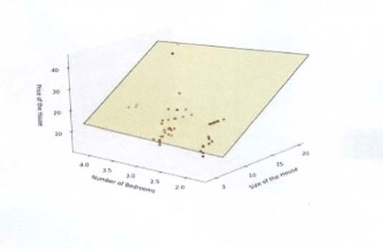
The above series of dots represents number of bedrooms and house sizes being conditioned against sale price. The yellow/greenish box is the regression line. The line is three-dimensional because we are dealing with a number of variables. In fact, the technology to display a regression line against many more variables has not been invented as of the writing of this article.
A problem of regression analysis is that it is a data hog. Since there are many variables or property characteristics that can cause or explain price differentials, there has to be a corresponding amount of data per each variable. If you have too many variables and not enough sales data, you run into the problem of ‘degrees of freedom.’ This is a fancy phrase that basically says one is asking too much from the data.
As a result, regression will allocate a penalty. As a rule of thumb, for every variable selected there should be seven to 10 sales.
Most appraisers would say that they are lucky enough to find five to 10 sales that might yield evidence regarding an injurious affection claim or the lack thereof. In those cases, the use of a qualitative and quantitative method known as ‘quality point’ might be the tool to use. The best example of this is in the textbook Property Valuation and Analysis, Second Edition, by RTM Whipple, published by Lawbook Co. 2006, ISBN #0 455 22394 7. A little closer to home is the book Readings in Canadian Real Estate, Fourth Edition, by Gavin Arbuckle and Henry Bartel, Captus University Publications, BSN #1-55322-062-5. There is an article entitled The Contemporary Direct Comparison Approach to Value” written many years ago by myself on the topic of dealing with small data bases using ‘quality point.’
Learn more about these advanced tools
Before running out and buying a shelf full of books on regression analysis, one is advised to take smaller steps and begin with books that deal with basic statistics and rudimentary data analysis. There are two reasons for this:
- Statistics has its own language and you need to understand it.
- Exploratory data analysis can reduce any good appraiser’s legs to jelly really fast. It will take you on a journey of self-discovery, not only on how you think about data, but its method of presentation and, most importantly, what the data is telling you.
If you want to learn more about regression analysis, please refer to the Regression Analysis Publications sidebar in the interactive electronic edition of Canadian Property Valuation (www.aicanada.ca).
Conclusions
Sophisticated real estate markets and claims of loss under the Expropriation Act need strong diagnostic tools to sort the ‘wheat’ from the ‘chaff.’ Regression modeling has its place in deciphering complex real estate problems. It is also fair to say that regression analysis is not easily applicable in every injurious affection case. Analyzing the outputs can be challenging, particularly in those cases where there is a marginal evidence for a claim. It can be complex, but so is the world of real estate data. Data does not reveal its secrets easily and even after ‘running’ a few regressions, it might show that the claim for injurious affection may be apparent, weak, or non-existent. At least with regression analysis, the real estate expert is closer to uncovering the truth based upon strong analytical skills.
It has often been said that the ‘simplest’ explanation of loss as a result of injurious affection is best presented so that arbitrators, judges and chairpersons can understand it. From my perspective, that statement has no significance, because we are living in a time where large blocks of data are readily available through the Internet. Conversations with American appraisers who deal in condemnation (land compensation claims) indicate that lawyers are heading back to school to get a better understanding of the use of data analysis, particularly regression analysis. Interesting reads include Statistical Evidence in Litigation by Will Yancey, PhD; Multiple Regression in Legal Proceedings, 80 Columbia Law Review 702, by Franklin M. Fisher; or Statistics for Lawyers and Law for Statisticians, 89 Michigan Law Review, by David H. Kaye.
I believe there is nothing more simple than the use of graphics to explain or defend a claim of injurious affection. However, the mathematics is needed to support the compensable amount.
Whether one likes statistics or not, they are gaining considerable momentum in the world of real estate analysis. For example, in some data analysis courses I recently took through COURSEA, there were 55,000 people taking primary courses on the topic.
Data analysis allows the practitioner to see real estate data patterns that were unthinkable 10 years ago. They afford glimpses to the makeup of data and how property variables aid in explaining variances in sale prices. After all, is that not the job of the real estate practitioner?
Learn more about regression analysis
If you want to learn more about regression analysis, you can start with the following award-winning books written by Dawn Griffiths and published by O’Reilly:
- Head First Statistics
- Head First Data Analysis
Since they might be in a PDF format, you can try www.headfirstlabs.com.
This material is very good because it treats the reader as if he or she knows nothing about statistics. There are numerous hand sketches and pictures. These books only delve into regression analysis on a simple basis. They are more designed to get you thinking about data analysis than specific tools for the job.
Another good source for statistical books and regression analysis is your local school board. The subject is taught in the senior years and is a very good starting point.
Books on regression analysis are often written at a very high level, however, the following books may be helpful:
- Multiple Regression: A primer, Paul D. Allison, Pine Forge Press. USBN # 0-7619-8533-6.
- Applied Regression Analysis, Linear Models, and Related Methods, John Fox, Sage Publications. USBN # 0-8039-4540-x.
- Correlation and Regression Analysis, A Historian’s Guide, Thomas J
Archdeacon, The University of Wisconsin Press. USBN#: 0-299-13650-7
Another good resource is COURSERA, an online program from universities around the world on a variety of topics including statistics. The nice thing about COURSERA is that it is free. However, do not think it is an easy ride. Many times there are 6-10 hours of homework per week, particularly if you want to earn a credit through the AIC.
There is no question that the book Quantitative Techniques in Real Estate
Counseling by Gene Dilmore is a must read, particularly since it deals with regression analysis in a number of chapters. Published by Lexington Books (ISBN #0-669-98251-2), it is an oldie and a goodie. Gene Dilmore was the person who coined the phrase ‘quality point’ and helped Dr. Graaskamp build the model we know today.