

What is the contributory value of a high-end swimming pool, cabana and landscaping
Canadian Property Valuation Magazine
Search the Library Online


Overview of the valuation problem
This was a question asked in a civil litigation matter dealing with a significant home that was improved with a very good quality pool, cabana and landscaping. The cost to install the swimming pool, landscaping and the cabana on the property was approximately $118,000. The pool, landscaping and cabana were installed in 2003 and 2004 and were only 4-5 years old at the date of the valuation.
In traditional real estate appraising, items such as pools, garages, etc. were supposed to be determined by using a paired sales analysis. In this process, the valuer needs to find several sales of the identical home to the one under appraisal, with the exception of the item to be valued. This method can be effective if identical homes can be found with at least one of them having the targeted physical characteristic.
Since there are no identical sales of houses selling in which a valuer can extract some type of contributory value for the item in question (e.g., pool, garage, etc.), then they would default to the next best set of data. The second set of data would be of sales that are not identical, but are similar to the property under appraisal. The valuer would then apply an adjustment in dollars to these items such as basement finishing, lot size in relation to the subject property, etc. The difference between the dollar adjustments of these items and the sale prices of the comparables would be the contributory value of the item. This process was repeated several times until there was a dollar difference between the sales that would show what a specific feature of a given house would be.
The problem with this secondary method is determining how the valuer adjusts for differences in lot size, basement finishing, etc., if there are no identical sales to be able to extract these differences from the market place. What really occurred is that the valuer makes a ‘judgement’ decision. Since these judgements are fraught with bias, it really has no place in proper valuation analysis. Unfortunately, this is a common problem when it comes to the valuation of real estate. Real estate practitioners need to seek out better vehicles to aid them in determining answers to complex real estate questions.
Suggested solution
The proper way to analyze differences in real estate data from the market place is through Regression Analysis. Regression Analysis has been in use for well over 100 years and is defined as “A statistical technique of finding a straight line between many data points.” Once the straight line has been determined, one can make predictions about the behaviour of people reacting in the real estate market place. There are two types of Regression Analysis. First, there is a Univariate model where one dependent variable is matched with an independent variable. An example of this is building size matched against sale price. We want to know the relationship between these to variables. Second, there is Multivariate where many variables are used in the model to aid in explaining price differences in properties. It is the latter model that we are dealing with in this article.
With Multivariate Regression Analysis, a large number of sales are put in a spreadsheet with all the variables that might influence price. Thus, each sale would have a selling price, area of house, area of basement finishing, age, lot size, garage, pool, no pool, hot tub, no hot tub, date of sale, cabana, shed, quality of landscaping around the pool area, pool age, location relative to backing onto green space, etc. In this analysis, the sales ranged in sale price from $400,000 to $1,000,000.
In the case of the subject property, we need sales that had a pool and sales without a pool. The same applies to the quality of the landscaping around the pool and the type of building by the pool. Regression Analysis requires a lot of information because it is being asked to determine the differences between data (e.g., with or without pools, landscaping, cabana/shed, etc.).
Unfortunately, Regression Analysis is not simply the process of putting data into a spreadsheet and pressing a button. Various relationships of the variables (e.g., house size, lot size, etc.) between the sale price of the houses need to be explored. The variables that do not play a large role in explaining the differences in the sale prices of the comparables are not used in the final analysis. This could be said for some of the variables considered. Since the valuer does not know what they are specifically, each variable needs to be examined on an individual basis. At this stage of the analysis, the valuer is trying to get a good balance between the actual data and the various variables that help to explain differences in price.
When the data is finally at a stage whereby the regression analysis becomes meaningful, then a series of observations can be made. We can first examine relations between houses with pools and houses without. Since we use a dummy variable (i.e., 1=house with pool and 0=house without a pool), we can graph these simple results to see if there is any difference between these two groups of data. The following is a graph showing a box plot between houses with pools and ones without. The box plot graph was invented by J. Tukey. The actual box is at the end of the first and third quartile, with the median shown as the black dot. The ‘whiskers’ are the T-lines of the data that are extended 3/2 times the inter-quartile range. The dots above that represent any outlying data points
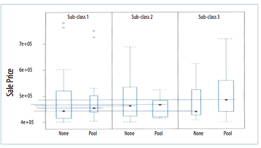
This graph shows three sets of data sub-classes. The reason why we did this analysis was to create a common data set within the main data sets of houses with and without pools that closely matched one another. On the left hand side of the box plots is sale price expressed in scientific notation. The 5e + 05 means 5 with 5 zeros or $500,000. The dotted blue lines are the expression of the box plot. The lines at the top of the blue lines which are horizontal are called ‘whiskers’” and represent 1.5 times the inter-quarantile figure of the data. The blue dots at the top are outlying sale prices
In sub-class 1. you see a black dot in the box which is labelled no pools. This is the median price of the homes. Beside that box is a smaller box of data with the pools. The black dot is shown to be higher. You can see this more clearly when you follow the blue line over to the sale price indicator. This indicates that, for this sub-class of data for houses with pools and ones without, houses with pools tend to sell for a higher price.
In sub-class 2, we see the same pattern. Houses with a pool sold for a higher value then ones that did not have a pool. The only difference between sub-class 2 and sub-class 1 is that the difference in terms of dollars is not as high.
In sub-class 3, we see a very wide dispersion between the median price of houses with pools and ones without.
This data is indicating volatility in the prices of houses with pools as opposed to without. If this were not so, we would see a more consistent price differential between houses with pools and ones without between all three sub-sets. The other factor is that one cannot extend the line of dots over to the sale price indicator and determine the difference in price. This cannot be done because he differences in the median prices of homes with pools and without pools is also due to other factors such as lot size, age, condition, etc.
The box plots are good visual tools that tell us there is a variance between houses with pools and ones without. This is a good indicator that something is going on between the data sets when it comes to pools. To be more exacting, only Regression Analysis can tell us what the final effect a pool has on price.
Multivariate Regression Analysis can be graphed, but because the coefficients produced by the model are so small, it is best to graph the coefficient (answer) to the standard error (how much one missed by). The following is the graph between the relationship between the returned coefficient of swimming pools and the standard error.
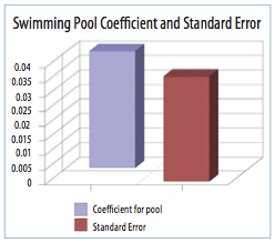
This graph is of the returned coefficient of houses with swimming pools against the standard error, or how much we missed by. We can see that the standard error is as large as the coefficient answer. This further reiterates that the real estate market is sending a strong mixed signal when it comes to swimming pools in backyards. Either the buyer wants them or not. There is no other message being sent by the buyer. Love them or leave them.
Regression Analysis produces a coefficient or value for each of the variables that are deemed to best explain price differentials. It also indicates the spread of this coefficient in terms of price. This is known as the standard error. The reason why there would be a spread in the coefficients is that there are always going to be some variances in the data. In the following data, we see the following Regression Analysis results.
Data set = pools, Name of Fit = L371 cases are missing at least one value.
Deleted cases are (8 56 74 51 3 95 68)
Normal Regression Kernel mean function = Identity Response = log[SP]
Terms = (ElapsdMths GarSF Hse_Age SiteSF QC NoFP IGPool Hse_Age^2 FBsmntSF HseSFHseSF^2 Pool_Age*IGPool)
Coefficient Estimates
Label estimate Std. Error t-value p-value Constant 12.8928 0.206721 62.368 0.0000
ElapsdMths 0.00194094 0.000773972 2.508 0.0144
GarSF 0.000110537 0.000103024 1.073 0.2869
Hse_Age -0.0124851 0.00399742 -3.123 0.0026
SiteSF 6.393998E-6 3.308006E-6 1.933 0.0572
QC 0.0803828 0.0235853 3.408 0.0011
NoFP 0.0152797 0.0192264 0.795 0.4294
IGPool 0.0404361 0.0362773 1.115 0.2688
Hse_Age^2 0.000291559 0.0000856595 3.404 0.0011
FBsmntSF 0.0000316127 0.0000214225 1.476 0.1445
HseSF -0.000196538 0.000105068 -1.871 0.0655
HseSF^2 4.490878E-8 1.613675E-8 2.783 0.0069
Pool_Age.IGPool -0.00148304 0.00198264 -0.748 0.4569
R Squared: 0.596208
Sigma hat: 0.0923906
Number of cases: 91
Number of cases used: 84
Degrees of freedom: 71
| R Squared | 0.596208 |
| Sigma hat | 0.0923906 |
| Number of cases |
Summary Analysis of Variance Table
| Source | df | SS | MS | F | p-value |
| Regression | 12 | 0.894859 | 0.0745716 | 8.74 | 0.0000 |
| Residual | 71 | 0.606058 | 0.00853602 |
Regression Analysis has an amazing ability to spew forth a considerable amount of data and analysis. We started by using 94 sales and, in the end, analyzed only 84. Some of the sales were eliminated because they sat outside of the normal distribution of data. In other words, some of the sales were not telling the valuer much about the data, so they were eliminated from the set. They are called outliers.
The model’s performance was not as one would have hoped for. The reason is that there is too much variability to be explained completely. However, that is the nature of data analysis. We found that the model was sending mixed signals in terms of the valuation of pools, in particular. This is not surprising given the fact that pools are generally real estate improvements that are shown to generate a considerable amount of controversy by buyers. Basically, with pools, either a buyer likes them or not. Many homeowners that have pools tend to fill them in. Other buyers see pools as a good way to entertain children from the ages of 5 to 15, for example.
In houses in the $400,000-plus range, pools might be an expected item. In other words, the buyer purchasing a $500,000-$800,000 house would most likely expect either a pool, attractive landscaping or a site that backs onto a green pace. Having all three items, for example, might interact with one another in a way that some of these attributes play a secondary role in explaining value.
We can say that pools do contribute something to the value of a property according to our data analysis. The attractive landscaping and building that seem to go with a pool do bolster value a bit. It would appear that landscaping and any pool building are integrated in with the pool in the eyes of the buyer. It seems to be the case that, if one was going to install a pool, it is best to have a pool with some added extra features, as opposed to a very plain pool. The time of year the property was sold with a pool was not a factor in terms of added value. It did not make a difference in terms of price.
The contributory value of a pool as taken from the Regression Analysis shows the following.
| COEFFICIENT | LOW ERROR | HIGH ERROR |
| 0.040 | 0.004 | 0.076 |
The coefficient of 0.040 can be expressed as a percentage of 4.0%. Thus, the lowest percentage would be 0.4% or a high of 7.6%. This means that the value of the pool could have a value 0.4% x the overall value of the house or 7.6% x the overall value of the house.
Obviously, the overall value of the house is a very important component to the end value of the swimming pool. If it was determined that the value of the house without the pool was $800,000, for example, then all we would have to do is apply the coefficients to that figures. When we apply our percentage values of the pool from the Regression Analysis, the contributory value of the swimming pool would be from a low of $3,200 to a high of $61,000. That is a considerable spread and reflects the volatile nature of this particular real estate asset. This is the same reading valuers have been receiving from buyers over the decades regarding swimming pools. To reiterate, buyers either love them or not. The dollar value of the range of swimming pools by the Regression Analysis is telling us the same thing, except it is expressing the fickle nature of pools in terms of dollars.
In the case of the subject property, the amount of depreciation that is inherent in the subject pool was $118,000 (cost new) – $50,000 (determined value) =$68,000. $68,000/$118,000 = 57%. Since the pool was five years old at the time of the valuation, we could easily say that 7% of the 57% is the result of physical depreciation and 50% for economic obsolescence. However, that is a matter of fine tuning.
As of the writing of this article, the matter is not settled. It is the age old argument when it comes to residential housing, in that most homeowners feel that, whenever large capital improvements are made to the house, the return is going to yield a 100% on the dollar of cost when the property is sold. This means that the other side needs to validate their position and bring to the table hard evidence to support their position that a swimming pool adds significantly to the overall value of the property. The author wishes them the best of luck with their task.