

An ‘across the fence’ approach for valuing a right of way across a hydro corridor
Canadian Property Valuation Magazine
Search the Library Online


An ‘across the fence’ approach for valuing a right of way across a hydro corridor
By George Canning, AACI, P. App
This case involves a 50-year-old house located in a good-sized community in Southwestern Ontario. The street is improved with varying housing types of differing ages as well as small apartment buildings. Some of the older houses have been torn down and replaced with more modern housing. The subject property and a high-tension transmission line owned by Ontario Hydro are located along the east side of the street. The hydro corridor also includes an easement in the middle of the line’s entire length. In order for the owners of the house to access the adjacent road, they had to drive underneath the physical hydro lines and on both the fee simple and easement lands owned by Ontario Hydro.
The executors of the property decided to market it. They quickly found that they did not have a Right of Way under the hydro lines or over the lands owned by Ontario Hydro, including the easement. The fact that the owners did this for 50 years negates this action for any other future homeowner according to their lawyer. The conclusion reached was that the property was landlocked and, without being granted a Right of Way by Ontario Hydro, the residential house and lot had virtually little or no value.
Ontario Hydro is clear in its policy regarding the valuation of a Right of Way, particularly over an existing hydro corridor. Their policy insists that an ‘across the fence’ or ‘best neighbors’ approach be used in the valuation of any proposed Right of Way. This method states that the estimate of the market value of the Right of Way is based upon the value of the adjacent land (house and lot) distinguished from the valuation of the Ontario Hydro corridor as a separate entity. It does not state where the comparables should be drawn from or imply any suggested method of valuation.
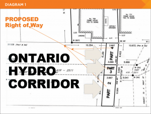
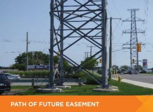
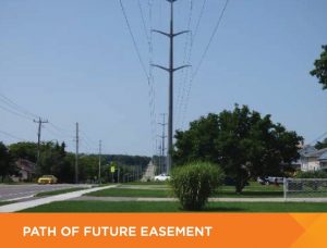
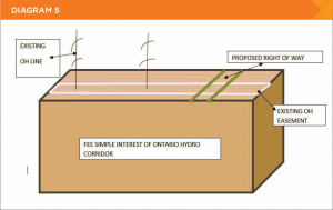
Below is a Diagram of the Ontario Hydro corridor and the house and lot behind it, as well as two images depicting the types of hydro towers on the corridor.
The proposed subject Right of Way is zoned residential and contains 729.8 square feet. Since the size of the proposed Right of Way is not large enough to be built upon, it calls into question the definition of market value. A bilateral monopoly now exists whereby there is only one buyer (the executors) and one seller (Ontario Hydro). In these situations, the seller is usually in the driver’s seat. However, we indicated to the executors that they were fortunate to be dealing with Ontario Hydro and not a private citizen. As such, the bilateral monopoly aspect of the proposed purchase of the Right of Way was eliminated and the standard definition of market value applied. A private citizen would not default to a ‘best neighbors’ or ‘across the fence’ approach, but would demand and get a high, non-reasonable payment for the proposed Right of Way, based upon the bilateral monopoly. As it turned out, Ontario Hydro treated the executors fairly and this real estate story ended happily.
Meanwhile, as a note, there has been a sale of a Right of Way on the same street as the subject property. It was a 1,786.88 square foot parcel that sold for $4,100 in 2008, which represented 75% of the Fee Simple interest of the entire lot to which this Right of Way was attached. Even though it is not comparable, it should be addressed in the report as an information item for the client.
Since we are using the ‘across the fence’ policy regarding the granting of a Right of Way over a utility corridor, the market value of the proposed Right of Way is, in part, the market value of the adjacent property. This property contains 11,712 square feet on which a house and garage is located. This would make sense, since the Right of Way is going to be attached to the 11,712 square foot existing parcel. The value of the proposed Right of Way is an extension of the existing lot and does not include the value of the house or garage. It assumes that the ‘across the fence’ site is unimproved. It is the land that is being extended with the proposed easement, not the buildings.
However, the problem still exists with this ‘across the fence’ approach to value because there have been no vacant lot sales which we have to interpret as also being ‘near to’ the subject property (11,712 square foot site). We need to create some type of a sales comparison methodology that would ‘best fit’ our subject property (11,712 square feet). Therefore, the valuer needs to focus on the known facts of the valuation of the Right of Way and the best way to proceed.
The appraisal problem: Determine the market value of a proposed Right of Way over an Ontario Hydro corridor that has an easement in its middle. Since the sales drawn from the marketplace for the valuation of the 11,712 square foot site are in Fee Simple, the actual acquisition of the Right of Way interest is not. How does one arrive at a different market value for the Right of Way if the land right interests are not the same?
Comparative sales: The comparable sales would best be drawn from similar types of older neighborhoods and not from newly created subdivisions, since those lots are not going to be improved with a similar end product found within older neighborhoods.
Method of sales analysis: Since we are dealing with the nebulousness of valuing a proposed Right of Way over an existing corridor, could the analysis of the sales data take on several forms? One method would simply examine a grouping of selected data without any formal adjustments (Method A). Therefore, the value of the Right of Way would be drawn from a composite of similar types of sales using central tenancy. Another method would be to execute a formal direct comparison approach (DCA) (Method B). We concluded that both methods would be used in the valuation process because they have an equal chance of being correct.
The site size of the sales should mirror as closely as possible the size of the existing site of 11,712 square feet, since the actual proposed Right of Way is an extension of this property. The comparable sites have to be fully serviced and zoned similar to that of the subject proposed easement.
Method A
Below are a number of sales of infill lots that have been selected for analysis.
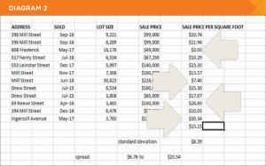
We can see that the average price is $15.15 per square foot of site area with a standard deviation of $8.39. This means that the spread around the average is between $6.76 and $23.54 per square foot. We cannot rely on the average sale price as a reliable number because of the wide spread in the variance of the data. The standard deviation is so wide because there are several outliers shown in red that are skewing the average. We removed these two outliers and ran the data again as shown below.
ADDRESS SOLD LOT SIZE SALE PRICE SP/PER SQ FT
398 Mill Street Sep-16 9,221 $99,000 $10.74
396 Mill Street Sep-16 8,289 $99,000 $11.94
517 Henry Street Jul-18 6,534 $67,250 $10.29
553 Leinster Street Dec-17 5,997 $140,000 $23.35
Mill Street Nov-17 7,368 $100,000 $13.57
Drew Street Jul-15 6,534 $100,000 $15.30
Drew Street Jul-15 3,808 $65,000 $17.07
394 Mill Street Dec-16 8,476 $85,000 $10.03
$14.04
Standard deviation: $4.52
Spread: $9.52 to $18.56
The average selling price per square foot of lot after removing the outliers is $14.04. The standard deviation is only $4.52, which means that the spread around the average is between $9.52 and $18.56. Although the attempt to smooth out the raw data is better, there still remains a dominating problem with the above data. The issue is the classic trend line due to the economies of scale between the sales.
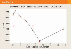
Below is a graph of the above data showing that, as lot sizes become smaller, the sale price per square foot of lot area gets larger and vice versa. The blue line in the graph is a LOWESS, which is a locally weighted smoother. It does exactly as its name implies.
The conclusion reached is that taking the average price of infilling residential lots and applying it to the property of 11,712 square feet does not make a lot of sense because the economies of scale and outlier sales are impacting too much on the average price.
Therefore, we have abandoned this approach (Method A) and applied a DCA (Method B) that can use quality point (QP) to efficiently deal with the data’s economy of scale.
For the sake of brevity, we used QP analysis as the basis for the DCA. Although, this article is about the valuation of a Right of Way, it is also an opportunity to demonstrate how QP handles two of the most difficult adjustments for any valuer: time and economies of scale.
Time
Time is just another predictor variable used in the analysis of real estate data. It is not special. In the traditional DCA, time is adjusted to all of the sales before the other adjustments are made to the comparables. In QP, we complete the before adjustments first and then do a time adjustment (if necessary). This is because there is no evidence that any valuer can justify a time adjustment (see Canadian Property Valuation article, Volume 61, Book 2, 2017) unless you are using multiple regression analysis (MRA). However, in QP, we can actually monitor the time adjustment and quantify its effect on the data. We can validate whether or not a time adjustment is warranted. It is cheaper and easier to do than running an MRA every time an appraisal is required. In QP, we monitor the effectiveness of our before adjustments through the mean adjusted selling price per square foot of lot size of the comparables (unit of comparison). The standard deviation (SD) of the mean of the adjusted selling price per square foot of lot size or unit of comparison is calculated before a time adjustment. The SD is expressed as a coefficient of variance percentage. In fact, it is a measure of the effectiveness of the predictor variables other than time.
In the valuation of the comparable lot sales, the selling price per square foot of lot before any adjustments was 127%. After applying all the ‘adjustments’ before any consideration regarding time, we were able to reduce the COV% of the adjusted selling price per square foot of lot size to 12%. The 12% is not an acceptable spread of the adjusted selling prices per square foot of lot of the comparables. Obviously, the missing predictor variable could be time. In this instance, we apply a time adjustment to the sales and monitor the effect of it via the COV, which is now at 12%. If we apply a time adjustment and it causes the COV% to decrease, then we keep adding a larger time adjustment percentage to see the results. In the report, it is shown as follows.
TIME ADJUSTMENT PER YEAR CHANGE (STARTING COV OF 12% BEFORE TIME)
1% NONE
2% NONE
3% LOWERED TO 10%
4% NONE
5% LOWERED TO 9%
6% NONE
7% LOWERED TO 8%
8% NONE
9% LOWERED TO 7%
10% NONE
11% LOWERED TO 6%
12% NONE
13% NONE
14% LOWERED TO 4%
15% NONE
16% NONE
17% NONE
We can see that the best time adjustment for this sale was 14% per year, since three tries after (15%, 16% and 17%) did not yield a response. This action reduced the COV from 12% to 4%, which is the goal of the DCA to reduce and explain the variation in the unit of comparison of the data. We cannot get the DCA model using QP to run more efficient.
Economies of scale (as part of the before adjustments)
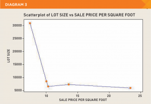
We had identified an issue with the sales in that there is an inverse relationship occurring with the unit of comparison (selling price per square foot of lot size). The bigger the site, the smaller the selling price per square foot of lot size, and vice versa. Below is a scatterplot of the sales data that demonstrates this market phenomenon.
Since QP uses a scale as a method of adjustment that rates the selected predictor variables, we can compensate for the effect of the economies of scale when it comes to the predictor variable lot size. All that is needed is to reverse the standard scoring of the predictor variables. The standard score is 1-4-9-16-25-36-49. In this instance, a 1 would now be a 49, and so on down the line. This means that a comparable property with a standard size lot that would normally be scored a 9 would be allocated the reverse score of a 25. This reversing action is nothing more that a re-expression found in typical statistic books dealing with data. Without this re-expression, the COV% would be 33% not 12% before any time adjustment.
The average lot size of the comparables is 11,840 square feet.
SALE NUMBER LOT SIZE SCORE (NORMAL) SCORE (REVERSE)
3 5997 4 36
1 6534 4 36
2 7368 4 36
4 8476 4 36
5 30,823 36 4
Validation of the correct adjustments to time and economies of scale
How does one know if this time and economies of scale adjustment method works? That is easy to see, since QP analysis has a residual testing feature built into the model. This simply predicts the actual selling of each comparable based upon the scores or ‘adjustments’ made to the predictor variables and compares the results to the actual selling prices of the comparables.
The testing process for the QP is extremely important because not all the scoring is based upon a mathematical average of the various attributes. Dr. Whipple of Curtin University in Australia said it best about the residual analysis of the QP model.
“Finally, residual analysis is a most important component of the technique. The assumption underlying the sales comparison approach is that recent buyer behaviour toward comparable sold properties will be the same as for the subject property. Residual analysis shows how well the model replicates the prices fetched for the comparable. If the replication is good, then the expectation is that it will produce an acceptable prediction of price for the subject property, if the analogy has been validly constructed. Few valuers test the logic they adopt on actual transactions. This method allows them to do so and is a desirable feature. The ultimate test of any method is the extent to which it produces results consistent with reality.”
– Property Valuation and Analysis, The Law Book Company Limited, 1995.
Below is the predicted Unit of Comparison (sale price per square foot of lot) shown in the third column against the actual selling prices of the comparable sales.
Index No. Actual Selling Price Predicted Selling Price Variance
Per Square Foot of Lot Area Per Square Foot of Lot Area
(After Quantitative Adjustments) (After All Adjustments)
1 $10.29 $10.51 2.14%
2 $13.57 $13.25 2.37%
3 $23.35 $21.72 6.94%
4 $12.84 $13.25 3.23%
5 $7.40 $7.76 4.89%
The QP model predicts the value of the five indexes within 2.14% to 6.94%. Since the scoring of the indexes has predicted a selling price per square foot of lot size residual of 3.91% on average, then the same scoring method can be applied to the subject property for a prediction of value. By then applying the same scoring method to the subject property as we did for the sales, the results show that the value of the subject property (not the easement) is as follows.
Predicted value range for the subject property
The prices per QP per square foot of lot area of the indexes were between $0.62 and $0.70 and are analyzed for their central tendency using the mean. This creates an average price per QP per square foot of lot area of $0.65. One standard deviation resulted in a $0.03 difference from the mean. In other words, the mean ($0.65) could also have a rate of ($0.65 + $0.03 = $0.68 or $0.65 – $0.03 = $0.62). The total weighted score of the subject property (23.40) is then applied against the mean price point per unit selling price to predict a value for the subject property (Method B).
Score of Subject Sale Price Per Square Lot Size Rounded to
Property (Method B) Foot of Lot Area of Subject
Per Quality Point Property 769
Parkinson Rd
23.40 x $0.62 x 11,712.00 = $170,000
23.40 x $0.65 x 11,712.00 = $178,000
23.40 x $0.68 x 11,712.00 = $186,000
Therefore, the value of the subject property (Method B) by the DCA is between $170,000 and $186,000. This equates to $14.52 to $15.88 per square foot of vacant lot area. This would be in Fee Simple and does not represent the market value range of the proposed Right of Way.
Right of Way rights versus Fee Simple rights
A Right of Way granted over a Fee Simple interest is nothing more than a physical plane of two dimensions: width and length. The Right of Way does not ‘take up’ some specified quantity of the Fee Simple because the Fee Simple interest is underneath the path of the Right of Way. In other words, the Right of Way is a surface right as opposed to an in-ground right for burying pipeline. The Fee Simple interest always stays intact. However, the placement of the Right of Way can disrupt that portion of the Fee Simple on which the Right of Way sits, depending upon the shape, angle and size of the Right of Way. As long as the Right of Way is situated along the edge of the site, it does not cause any diminution in value by having the Right of Way in place. In the case of the subject property’s proposed Right of Way over the Ontario Hydro corridor, there is no change in the Fee Simple and easement right of the existing Ontario Hydro lands. In other words, the proposed Right of Way is not a burden on the Ontario Hydro lines because it simply sits on top of the existing land and easement. Since the Right of Way is something that is added to the underlying Fee Simple interest of the Ontario Hydro lands, its value would automatically reflect some portion of the value of the Fee Simple right.
Below is a view of the Ontario Hydro corridor with its own central easement with the proposed Right of Way going crossways over the corridor.
There have been considerable volumes written on the topic regarding the difference in market value between the Right of Way interest and the Fee Simple interest. The value of the Right of Way is often expressed in the marketplace as a percentage of the Fee Simple (50% to 100%). We know that an existing Right of Way was paid on the subject street using a 75% contributory value of the Fee Simple. A good article on this topic is Nonlinear Effects on Easements Valuations by Henry J. Munneke and Joseph A Trefzger. It can be found in the Journal of Real Estate Research, Volume 16, Number 2, 1998, as well as on the Internet.
We have elected to use a 75% rate against the Fee Simple. This means that the market value of the proposed subject Right of Way is 75% of $14.52 to $15.88 or $10.89 to $11.91. When these rates are applied to the subject Right of Way area of 729.8 square feet, a value range from $7,948 to $8,692 emerges.
As a footnote, we cannot compare the Right of Way rate of $2.29 paid (1,787 square feet) for a Right of Way along the same subject street several years ago. The reasons are twofold:
A) There is a difference in time of 10 years between sales of a Right of Way on the subject street. There has been an acceleration of residential real estate prices that are beyond anyone’s estimations. This increase in the improved residential marketplace would also spill over into the market for vacant residential lots
B) The difference in the sizes of the two Rights of Way: 729.8 square feet (subject) compared to 1,787 square feet. As seen within the DCA, site size was shown to have an inverse relationship with the larger site having a smaller per square foot sale price and the smaller site having a larger one. The same applies when comparing the two sizes of the Rights of Way. The subject’s Right of Way is significantly smaller and, therefore, would have a much larger per square foot rate overall.
The bottom line is that there is no real comparison between the amount paid for the Right of Way on the subject street to that of the subject Right of Way.
The conclusion reached was that the market value of the subject easement was worth $10.96 per square foot of the easement of 729.8 square feet. This equates to $8,000. Ontario Hydro accepted this value of the easement and an easement of access was granted to the executors of the property. The executors subsequently sold the house and lot.